Generative art. Deconstructed image explained in detail.
Deconstructed
What is image deconstruction?
Societies have used the concept of “deconstruction” in different cultural categories, from philosophy[1], architecture [2] or more recently food[3]. The idea behind Image deconstruction is to take the digital constituents of an image, the pixels, and explore the artistic value of rearranging them according to some criteria. Image deconstruction starts with a pre-existing digital image of a piece of art and an algorithm rearranges the position of the pixels. The criterion used in this first collection is color smoothness throughout the image. We can measure this degree of color smoothness by defining some mathematical expression that quantifies the value of the whole image.
Let’s define smoothness as energy
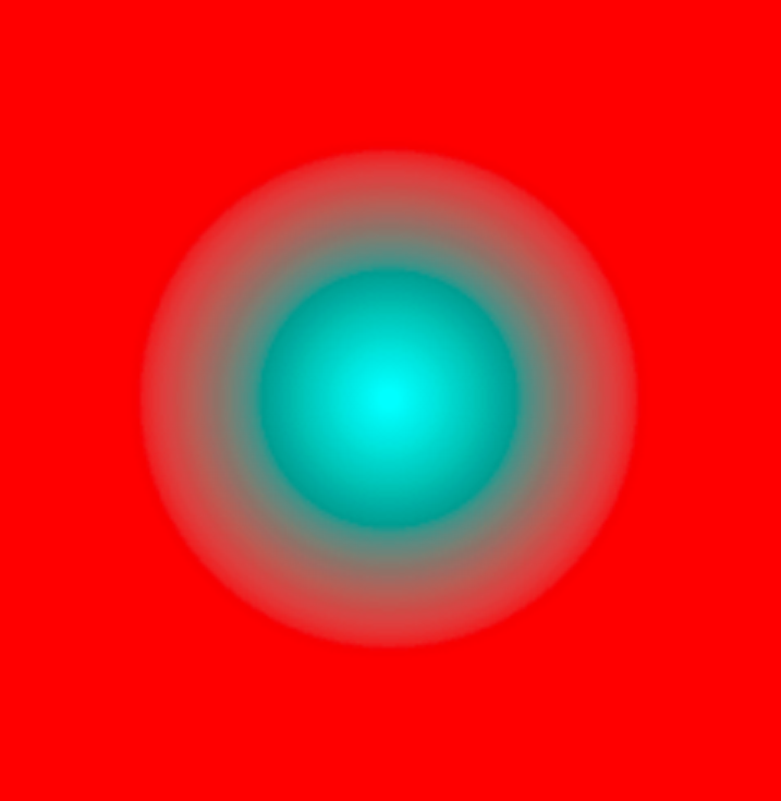
For simplicity, let us name the overall smoothness of the image as its energy. An intrinsic characteristic that can be quantified with accuracy. What does it mean that an image, in this context, has low energy? It means that each pixel of the image is surrounded by pixels of a similar colour. On the opposite side, a high energy arrangement of the pixels would look like random pixels, like noise. This due to the fact that any emerging pattern has been broken, and our visual system would fail to identify anything relevant. We can see it in these two examples:

Once we sketched this concept of image energy, our aim is to find the pixel configuration or arrangement with maximum color smoothness, i.e. with the lowest energy. A possible brute force approach is to consider all possible arrangements in an image, measure them and get the smallest one.
Astronomical complexity of deconstructed image and beyond
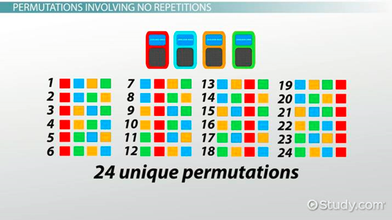
It is time to discover the complexity of all possible pixel arrangement in an image. Let us consider a trivial example of an image with 4 distinct pixels: red, blue, yellow and green. The picture below shows the 24 possible ways to arrange them. In mathematical terms, the way in which we can combine 4 elements in ordered groups of 4 (ordered meaning that their location matters) we call it permutations of 4 elements without repetition.
For an image with N pixels, the number of possible arrangements is:
When we try to calculate this number of combinations for very small square images
-
2x2 pixels → 24
-
3x3 pixels → 362,880
-
9x9 pixels → (wait we may need two lines) 5797126020747367985879734231578109105412357244731625958745865049716390179693892056256184534249745940480000000000000000000
We can express the very large number above in a more manageable way as 5.7e120, meaning that it has 120 digits. It becomes astonishing the astronomical growth of this progression, where a simple 9x9 pixels image has more permutations than the estimated number of particles in the universe. The famous low-resolution crypto punks [4] with images of 24x24 pixels will yield a number of permutations of 4e1341, an unimaginable number.
Illustrating this absurd in more real-life image sizes:
-
15000 pixels→ 2e+56129
-
0.15 Mpixels → 3e+711272
-
1.5 Mpixels [5] → 4e+8612698
These are numbers only in the realm of mathematics.
Once it is clear that the number of possibilities is humongous, we must note that most of these combinations lead to high energy images. If we randomly choose a permutation, it is going to show high energy. Only very rare arrangements lead to low energy images (low energy meaning 10% of the energy of a random permutation). Unfortunately we have just learned that the search space is immense. Finding the absolute minimum by brute force is impossible once the image is larger than a few pixels. While perhaps a quantum computer can solve this problem in the future, an approximate method, namely a meta-heuristic method, will help us find needles in a haystack.
Background of my story with Deconstructed Image
Despite art has been around early in my life (my father painting is in my earliest memories), I have developed a technical career with special interest in engineering, physics and computation. Programming and modelling of physical problems, together with photography is something I always found passion doing.
It has been roughly 15 years that I became really interested in the science of color and started experimenting with perceptual color spaces like L*a*b*[6]. A few years later I became familiar with meta-heuristic techniques as a way to solve image combinatorial problems.
When recently blockchain technologies, NFTs and the concept of generative art became part of my interest, the willing of being part of that grew up, and the idea of Image deconstruction started to build up.
It took me many months to shape, and do it in parallel with the other two pillars of my artistic project. It took a lot of my free time during the pandemic. I spent many of those hours optimizing the code and trying to understand the peculiarities of the algorithm and scaling. Even by using meta-heuristics techniques the problem was too complex to solve it without cache techniques and code optimization.
Deconstructing an image. How does it work?
There may be specific technical documentation, or even the full source code to generate deconstructed images. This depends on the interest of the community on this technique. Yet I wanted to give some overall description on how the generative process occurs.
Computing energy
First it is important to define exactly how to compute the energy of the image. We assess color smoothness by adding up color differences among each pixel and its neighbors. Most of the images we see in the digital world come in the form of RGB images, where color encoding using 3 componentes: red (R), green (G) and blue (B). Each of these 3 numbers typically ranges between 0 and 255. Th (R,G,B) triplet defines the color of the pixel. If we want to measure the color difference between two pixels: (R1, G1, B1) and (R2, G2, B2), we could simply calculate the Euclidian distance:
The color space RGB is very intuitive but it is not well suited to calculate perceptual differences. This means that two color differences maybe numerically identical but radically different for a human observer. Another less known (and not intuitive) color space is L*a*b*. We can transform RGB images to this new color space and each pixel will have a triplet (L1, a1, b1). The color difference formula in this new space will be better to match numerical values and human perception:
Now that we know how to calculate the difference of color between two pixels, the graph below illustrates how to calculate the energy of the whole image. Each of the yellow arrows imply a color difference, calculated as in the above formula.
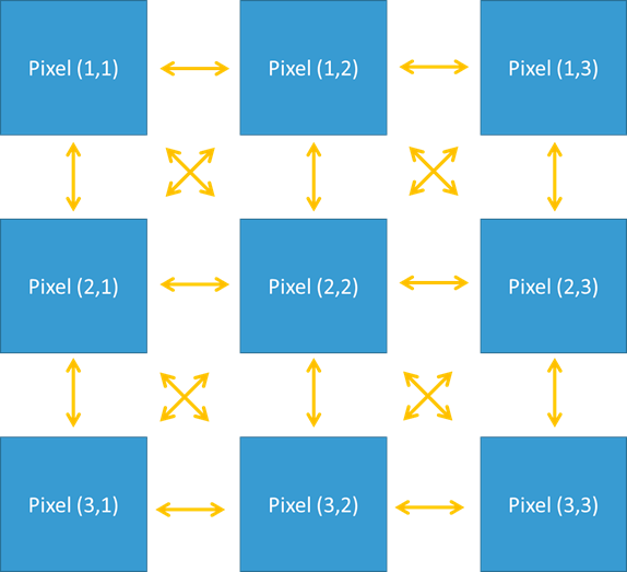
The energy of the image will be the sum of all yellow arrows. Note that color differences are only calculated once, i.e. if we account for the difference between pixel(1,1) and (2,2), we do not add up the reciprocal one (pixel(2,2) and pixel(1,1)).
Reducing the energy
Now that we know how to calculate the energy of the complete image, the task is to reduce it by changing pixel locations. This task is done using an adaptive simulated annealing (ASA) algorithm. The algorithm does not follow exactly the concepts described by Lester Ingber[7] (who invented ASA), as I failed to take profit of his implementation proposal for this particular problem. Finally a slightly different adaptive approach was implemented that led to faster and more predictable results than the standard simulated annealing (SA) algorithm.
Simulated annealing
The approach, in very simple terms, consists of:
- Swapping randomly two pixels and evaluating if that produces overall a better (lower energy) or worse result (higher energy).
- If the change produces a better result it is accepted, and the iteration starts again.
- If the change produces a worse result it will be accepted “sometimes”. The likelihood of accepting a worse change is governed by a parameter called temperature.
The whole algorithm (simulated annealing) gets inspiration in the annealing processes in metals. A slow cool-down produces better atomic arrangements than a fast cool down.
At the initial stages, the temperature is high (worse changes are widely accepted) and eventually we reduce the temperature (worse changes are not accepted). One key element of the success is how to reduce the temperature (when, how much, for how long, etc…).
In my experience the best solutions require a full shake out of the pixels or full randomization as a first step. We do that either starting at a high temperature or pre-shuffling the pixels before the optimization starts. Eventually the quality of the solution (low energy) depends on the number of iterations and the right cooling approach.
One final thought goes to the pixels in the border of the image, as they will have less neighbors than the internal pixels. To circumvent this limitation a continuity condition is a posibility. In such case, the generated images will naturally tile up placing a copy of the optimized image on the right, the left, up or down. This can be a beautiful add-on.
The final result shown in the NFTs comes in two different forms. In the simplest we have one the final image, with extraordinary low energy. In the second form we enjoy a movie of the transition from the original image and the annealing process.
Update 2025
During 2024 and 2025 I embarked myself into further optimization of the algorithm. You can read about my journey here.
Video of the process
References
[1] https://en.wikipedia.org/wiki/Deconstruction
[2] https://en.wikipedia.org/wiki/Deconstructivism
[3] https://movingwithmitchell.com/2018/01/31/dessert-deconstructed-postre-deconstruido/
[4] https://www.larvalabs.com/cryptopunks
[5] https://mrob.com/pub/comp/hypercalc/hypercalc-javascript.html
[6] https://en.wikipedia.org/wiki/CIELAB_color_space
[*] https://www.geeksforgeeks.org/maths/permutation/
#deconstructedimage #imagedeconstruction #generativeart #simulatedannealing #algorithm #optimization #innovation